Google Sheets

Celonis does not warrant the availability, accuracy, reliability, completeness, or usefulness of any information regarding the subject of third-party services or systems.

With Google Sheets modules in Boost.space Integrator, you can manage rows, cells, sheets, spreadsheets, values, and conditional formats in your Google Sheets account.

To use Google Sheets with Boost.space Integrator, you must have a Google account. If you do not have one, you can create one at accounts.google.com. To use instant trigger modules, you must have the Boost.space Integrator Google Sheets extension.

Refer to the Google Sheets API documentation for a list of available endpoints.

Connect Modules Using the Google Account Sign In

To connect Google Sheets to Boost.space Integrator, you must first connect your Google account.

1. Log in to your Boost.space Integrator account, add a Google Sheets module to your scenario, and click Create a connection.
2. Optional: In the Connection name field, enter a name for the connection.
3. Click the Sign in with Google button and select your Google account.
4. Review the access information and click Allow.

You have successfully established the connection. You can now edit your scenario and add more Google Sheets modules. If your connection requires reauthorization at any point, follow the connection renewal steps here.

Set Up Google Sheets Webhooks

Caution: The Make Google Sheets Add-on is currently not available because of Google’s restrictions, and the following procedure should be followed to use the Perform a Function and Watch Changes instant modules.

To use the Google Sheets Perform a Function or Watch Changes instant modules, you must first paste a script and your module’s webhook address into your spreadsheet. Follow the steps below to do so.

To set up the webhook:

1. Log in to your Boost.space account, add either the Perform a Function or Watch Changes module to your scenario, and click Create a webhook or Add.

2. Optional: Enter a name for the webhook in the Webhook name field.

3. Click Save.

4. Next you will paste a script into your spreadsheet. Click here to access the script and copy the entire content.

5. Open the spreadsheet and go to Extensions > Apps Script. You will see a new project containing default content.

6. Delete the default content and paste the script you copied in Step 4. This script must be updated with the webhook address from your Google Sheets module.

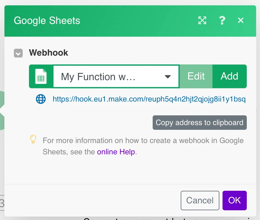
7. To obtain the webhook address, go back to your scenario, click on the module, and click Copy address to clipboard.

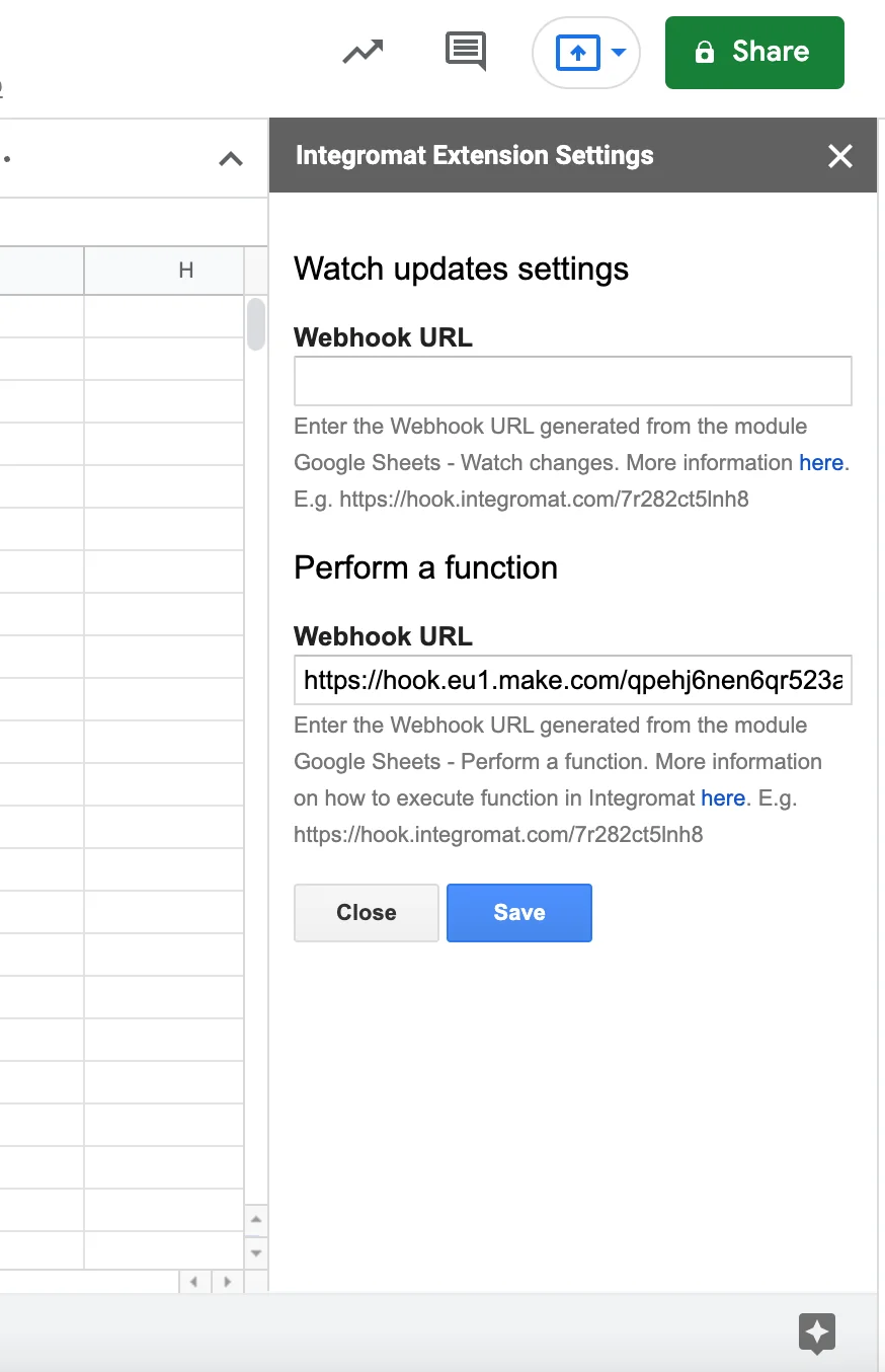
8. Now return to the Apps Script project in your spreadsheet. At the beginning of the script, you will see the lines WATCH_CHANGE_WEBHOOK_URL = 'https://hook.eu1.make.com/xxx'; and PERFORM_FUNCTION_WEBHOOK_URL = 'https://hook.eu1.make.com/xxx';.

9. Depending on the module you are using, replace https://hook.eu1.make.com/xxx with the webhook address you copied in Step 7.

   Caution: It is important to paste the full webhook address into the script to avoid any errors.

10. Click the Save icon.

11. In the left sidebar, click the Triggers icon.

12. Click Add Trigger.

13. In the Select event type field, select On edit, and click Save.

14. If prompted, authenticate your account and confirm access.

The Perform a Function or Watch Changes module will now send data through the webhook when the selected event occurs.

Did you know?

You can find over 100 predefined Google Sheets sample templates here.

After connecting the app, you can perform the following actions:

Triggers

Watch Rows

Retrieves values from every newly added row in the spreadsheet.

The module retrieves only new rows that have not been filled in before. The trigger will not process an overwritten row.

Connection

Establish a connection to the spreadsheet using your Google account.

Choose a Method

Select a method to choose the spreadsheet whose rows you want to watch.

Choose a Drive

Select Google Drive, where you have the spreadsheet whose rows you want to watch.

Spreadsheet ID

Choose the Spreadsheet ID whose rows you want to watch.

Spreadsheet

Select the spreadsheet that contains the sheet you want to watch.

Table contains headers

Select whether the spreadsheet contains the header row. If the _Yes_option is selected, the module doesn’t retrieve the header row as output data, and variables in the output are then called by the headers. If the _No_option is selected, the module retrieves the first table row, and the output variables are called simply A, B, C, D, etc.

Row with headers

Enter the range of the header row, e.g., A1:F1.

Value render option

Formatted value

The values in the reply will be calculated and formatted according to the cell’s formatting. Formatting is based on the spreadsheet’s locale, not the requesting user’s locale. For example, if A1 is 1.23and A2 is =A1 and formatted as currency, then A2 will return "$1.23".

Unformatted value

The values will be calculated but not formatted in the reply. For example, if A1 is 1.23 and A2 is =A1 and formatted as currency, then A2 will return the number "1.23".

Formula

The values will not be calculated. The reply will include the formulas. For example, if A1 is 1.23 and A2 is =A1 and formatted as currency, then A2 will return "=A1".

Date and time render option

Serial number

Instructs date, time, datetime, and duration fields to be outputted as doubles in “serial number” format, as popularized by Lotus 1-2-3. The whole number portion of the value (to the left of the decimal) counts the days since December 30th, 1899. The fractional portion (to the right of the decimal) counts the time as a fraction of the day. For example, January 1st, 1900 at noon would be 2.5. 2 because it’s 2 days after December 30th, 1899, and .5 because noon is half a day. February 1st, 1900 at 3 pm would be 33.625. This correctly treats the year 1900 as not a leap year.

Formatted string

Instructs date, time, datetime, and duration fields to be outputted as strings in their given number format (which depends on the spreadsheet’s locale).

Limit

Set the maximum number of results that Boost.space Integrator will work with during one execution cycle.

Watch Changes

This module watches for changes in all the cells of a spreadsheet. It means that when you update numerous cells in one row, one by one, Boost.space Integrator will then receive multiple updated events.

Webhook

Establish a connection to the spreadsheet using the Make.com add-on.

Perform a Function

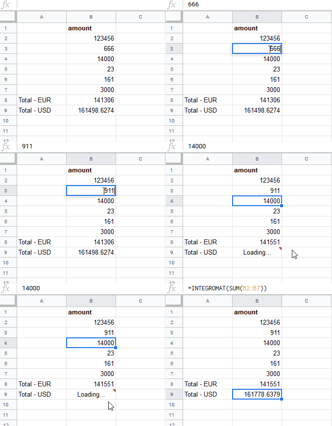
Boost.space Integrator allows you to use the custom function MAKE in Google Sheets similarly to built-in functions like AVERAGE, SUM, etc. It allows you to perform the function in Boost.space Integrator and return the result back to the sheet. The function MAKE accepts as many parameters as you need.

Perform a Function Example

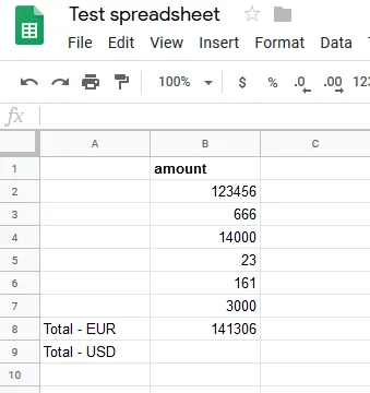
Sample sheet

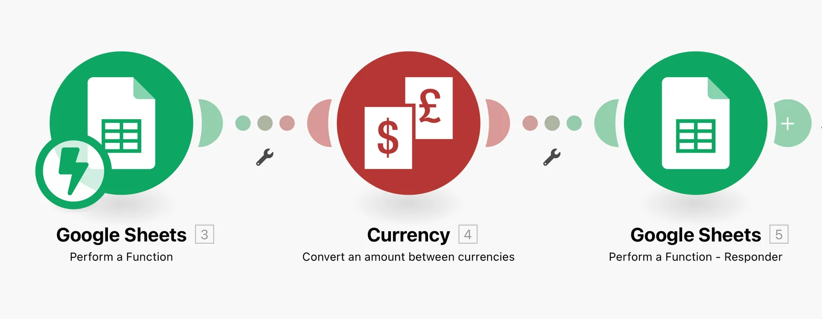
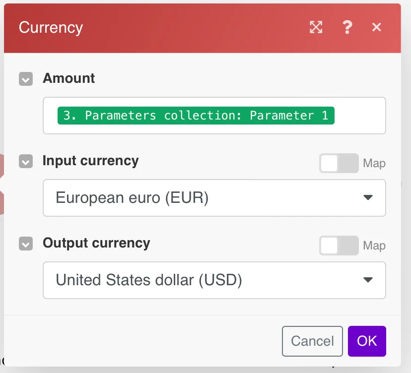
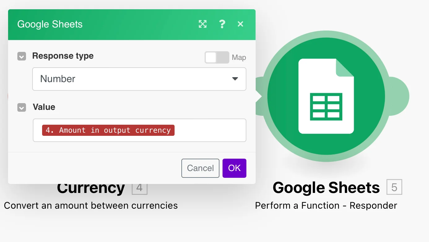
The Total – EUR amount SUM will be converted, according to the current exchange rate, to the Total – USD amount and will be inserted into the desired field using Boost.space Integrator.

1. Create a scenario. Use the following modules:

   • Google Sheets > Perform a Function
   • Currency > Convert an Amount between Currencies
   • Google Sheets > Perform a Function – Responder

   

   1. Google Sheets > Perform a FunctionGenerate a webhook and paste it into the Make.com add-on in Google Sheets.

      

   2. Currency > Convert an Amount between CurrenciesConverts the mapped EUR amount to USD.

      

   3. Google Sheets > Perform a Function – ResponderInserts the converted amount into the sheet cell.

      

2. Run the scenario

3. Enter the MAKE function into the desired cell to load the converted amount.

   

   When the user changes the amount, the MAKE function re-calculates the Total – USD according to the current exchange rate:

   

How to perform a custom function?

You can simply use the function like built-in functions in Google Sheet.

Create a new scenario with the following modules:

• Perform a Function – the module receives the parameters passed to the function
• Perform a Function – Responder – the module returns the result of the function execution back to the sheet

Webhook URL

Establish a connection to the spreadsheet using the Make.com add-on.

Actions

Add a Row

Adds a row to a sheet.

Connection

Establish a connection to the spreadsheet using your Google account.

Choose a Method

Select an option to choose the spreadsheet in which you want to add a row.

Choose a Drive

Select Google Drive to choose the spreadsheet in which you want to add a row.

Spreadsheet ID

Enter the Spreadsheet ID in which you want to add a row. Alternatively, you can search the spreadsheet by clicking Search Spreadsheets.

Spreadsheet

Select the Google spreadsheet.

Sheet Name

Enter a sheet name in which you want to add a row.

Column range

Select the column range that you want to work with.

Unformatted

Select or map whether to insert a row unformatted.

Values

Enter (map) the desired cells of the row you want to add.

Value input option

User entered

The values will be parsed as if the user typed them into the UI. Numbers will remain numbers, but strings may be converted to numbers, dates, etc., following the same rules that are applied when entering text into a cell via the Google Sheets UI.

Raw

The values the user has entered will not be parsed and will be stored as-is.

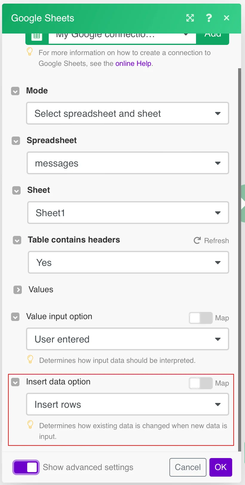
Insert data option

Insert rows

Rows are inserted for the new data.

Example

What happens when the Insert rows option is selected (the _Add a Row_module is executed 3 times):

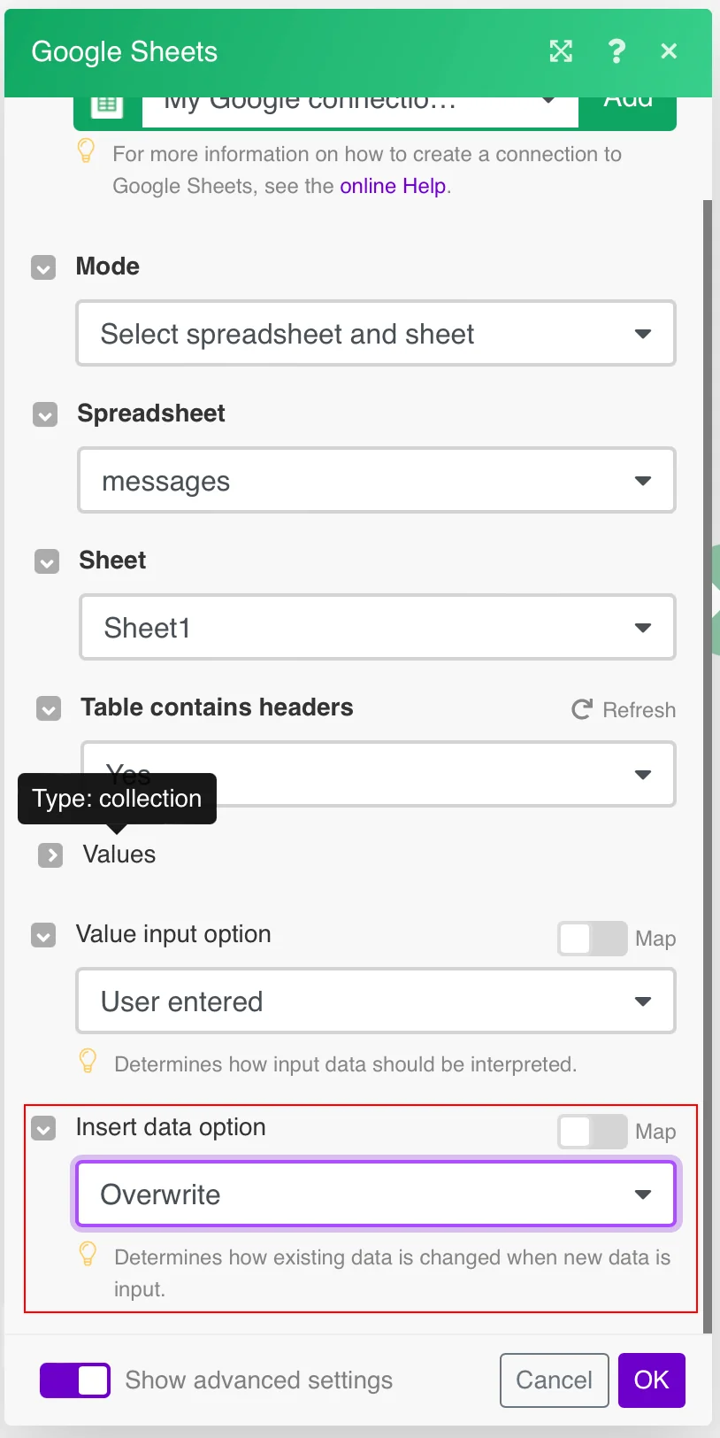
Overwrite

The new data overwrites the existing data in the areas where it is written. (Note: adding data to the end of the sheet will still insert new rows or columns so the data can be written.)

Example

What happens when the Overwrite option is selected (the _Add a Row_module is executed 3 times):

Update a Row

This module allows you to change the cell content in a selected row.

Connection

Establish a connection to the spreadsheet using your Google account.

Choose a Method

Select an option to choose the spreadsheet whose rows you want to update.

Choose a Drive

Select Google Drive to choose the spreadsheet whose rows you want to update.

Spreadsheet ID

Enter the Spreadsheet ID whose rows you want to update. Alternatively, you can search the spreadsheet by clicking the Search Spreadsheets.

Spreadsheet

Select the Google spreadsheet.

Sheet

Select the sheet you want to update a row in.

Row number

Enter the number of the row you want to update.

Values

Enter (map) the values in the desired cells of the row you want to change (update).

Value input option

User entered

The values will be parsed as if the user typed them into the UI. Numbers will remain numbers, but strings may be converted to numbers, dates, etc. following the same rules that are applied when entering text into a cell via the Google Sheets UI.

Raw

The values the user has entered will not be parsed and will be stored as-is.

Clear a Row

Deletes values from a specified row.

Connection

Establish a connection to the spreadsheet using your Google account.

Spreadsheet

Select the Google spreadsheet.

Sheet

Select the sheet you want to delete data from.

Row number

Enter the number of the row you want to delete, e.g. 23.

Delete a Row

Deletes a specified row.

Connection

Establish a connection to the spreadsheet using your Google account.

Spreadsheet

Select the Google spreadsheet.

Sheet

Select the sheet you want to delete a row from.

Row number

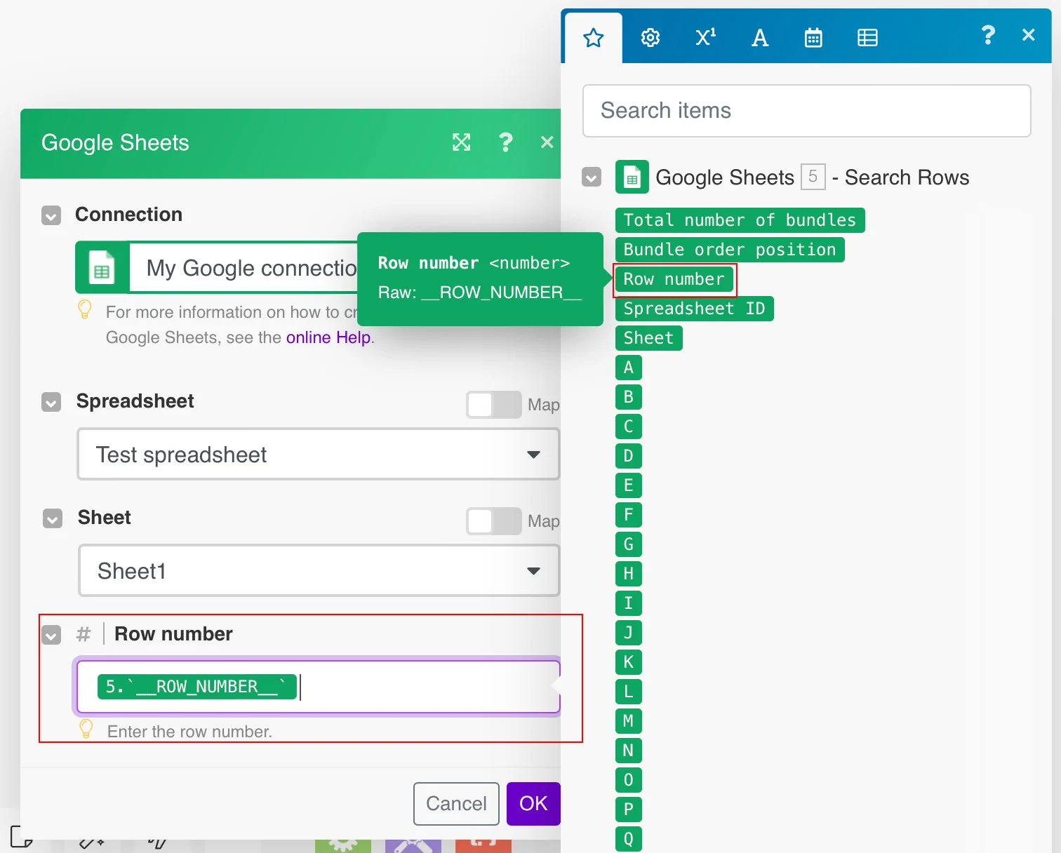
Enter the number of the row you want to delete, e.g. 23 or map the number from a preceding module, e.g. Search Rows.

Get a Cell

Retrieves a value from a selected cell.

Connection

Establish a connection to the spreadsheet using your Google account.

Spreadsheet

Select the Google spreadsheet.

Sheet

Select the sheet that contains the cell you want to retrieve data from.

Cell

Enter the ID of the cell you want to retrieve data from, e.g. A6.

Update a Cell

Connection

Establish a connection to the spreadsheet using your Google account.

Spreadsheet

Select the Google spreadsheet.

Cell

Enter the ID of the cell you want to update, e.g. A5.

Value

Enter the new value.

Value input option

User entered

The values will be parsed as if the user typed them into the UI. Numbers will remain numbers, but strings may be converted to numbers, dates, etc., following the same rules that are applied when entering text into a cell via the Google Sheets UI.

Raw

The values the user has entered will not be parsed and will be stored as-is.

Clear a Cell

Deletes a value from a specified cell.

Connection

Establish a connection to the spreadsheet using your Google account.

Spreadsheet

Select the Google spreadsheet.

Sheet

Select the sheet you want to delete a cell from.

Cell

Enter the ID of the cell you want to delete, e.g. A5.

Add a Sheet

Creates a new sheet in a selected spreadsheet.

Connection

Establish a connection to the spreadsheet using your Google account.

Spreadsheet

Select the Google spreadsheet.

Properties

Title

Enter the name of the new sheet.

Index

Enter the sheet position. The default is 0 (places the sheet in the first place).

Create a Spreadsheet

Connection

Establish a connection to the spreadsheet using your Google account.

Title

Enter the name of a new spreadsheet.

Locale

The locale of the spreadsheet in one of the following formats:

• an ISO 639-1 language code such as en,
• an ISO 639-2 language code such as haw, if no 639-1 code exists,
• a combination of the ISO language code and country code, such as en_US.

Recalculation interval

The amount of time to wait before volatile functions are recalculated:

On change

Volatile functions are updated upon every change.

On change and every minute

Volatile functions are updated upon every change and every minute.

On change and hourly

Volatile functions are updated upon every change and hourly.

Time zone

Select the time zone of the spreadsheet.

Number format

Select the default format of all cells in the spreadsheet.

TEXT

Text formatting, e.g 1000. 12

NUMBER

Number formatting, e.g, 1,000.12

PERCENT

Percent formatting, e.g 10. 12%

CURRENCY

Currency formatting, e.g $1,000.12

DATE

Date formatting, e.g 9/26/2008

TIME

Time formatting, e.g 3:59:00 PM

DATE time

Date+Time formatting, e.g 9/26/08 15:59:00

SCIENTIFIC

Scientific number formatting, e.g 1. 01E+03

Sheets

Add sheets to the new spreadsheet.

Perform a Function – Responder

This module is to be used together with the Perform a Function module.

Response type

Select whether you insert text or a number into the sheet.

Value

Map the value from the previous module you want to insert into the sheet.

Delete a Sheet

Deletes a specified sheet from a spreadsheet.

Connection

Establish a connection to the spreadsheet using your Google account.

Spreadsheet

Select or map the Google spreadsheet that contains the sheet you want to delete.

Sheet

Select or map the sheet you want to delete.

Make an API Call

Allows you to perform a custom API call.

Connection

Establish a connection to the spreadsheet using your Google account.

URL

Enter a path relative to https://sheets.googleapis.com/v4/.

For example: /spreadsheets/{{spreadsheetID}}.

Method

Select the HTTP method you want to use:

• GET – to retrieve information for an entry.
• POST – to create a new entry.
• PUT – to update/replace an existing entry.
• PATCH – to make a partial entry update.
• DELETE – to delete an entry.

Headers

Enter the desired request headers. You don’t have to add authorization headers; we already did that for you.

Query String

Enter the request query string.

Body

Enter the body content for your API call.

Example of Use – Get Spreadsheet

The following API call returns specified spreadsheet details.

URL:

/spreadsheets/{{spreadsheetID}}

Method:

GET

The result can be found in the module’s Output under Bundle > Body:

Create a Spreadsheet from a Template

Creates a new spreadsheet from a template sheet.

Connection

Establish a connection to your Google Sheets account.

Enter a Template Spreadsheet ID

Select or map the Template Spreadsheet ID from which you want to create the spreadsheet.

Choose a Drive

Select or map the drive where you want to create the spreadsheet.

Template Spreadsheet ID

Select the template from which you want to create the spreadsheet.

If the spreadsheet contains tags like {{name}}, they are retrieved below.

Your file MUST contain at least one tag for this module to work.

Title

Enter a name for the spreadsheet.

New Drive Location

Select or map the drive to store the new spreadsheet.

New Document’s Location

Select or map the folder, where the new spreadsheet should be placed.

Copy a Sheet

Copies a sheet to another spreadsheet.

Connection

Establish a connection to your Google Spreadsheets account.

Choose a Method

Select or map the option to choose the spreadsheet that you want to copy.

Choose a Drive

Select or map the drive location where the spreadsheet that you want to copy is located.

Spreadsheet ID

Select or map the Spreadsheet ID you want to copy.

Destination Drive Location

Select or map the drive location where you want to store the copied spreadsheet.

Destination Spreadsheet ID

Select or map the copied Spreadsheet ID.

Clear Values from a Range

Clears a specified range of values from a spreadsheet.

Connection

Establish a connection to your Google Spreadsheet account.

Enter a Spreadsheet ID and Sheet Name

Select an option to choose the spreadsheet and sheet name whose value you want to clear.

• Enter manually
• Select from all
• Select by path

Spreadsheet ID

Enter the Spreadsheet ID from which you want to clear the values.

Sheet Name

Enter a sheet name from which you want to clear the values.

Range

Enter the range you want to get. For example, A1.

Add a Conditional Format Rule

Creates a new conditional format rule at the given index. All subsequent rules indexes are incremented.

Connection

Establish a connection to your Google Spreadsheets account.

Enter a Spreadsheet and Sheet ID

Select an option to choose the spreadsheet and sheet name to which you want to create a format rule.

• Enter Manually
• Select from all
• Select by path

Spreadsheet ID

Enter the Spreadsheet ID to which you want to create the conditional format rule.

Sheet ID

Enter the Sheet ID to which you want to create the conditional format rule.

Range

Enter the range of rows and columns to which you want to apply the conditional rule format. For example, A1.

Index

The zero-based index where the rule should be inserted.

Format Rule

Select or map the rule for the conditional format rule.

Condition

Select or map the condition and enter the value for the format rule. For more information, see the boolean and gradient conditions.

Cell Format

Select or map the cell background color.

Text Format

Set the text format such as foreground color, bold, italic or strikethrough.

Delete a Conditional Format Rule

Deletes a conditional format rule at the given index. All subsequent rule indexes are decremented.

Connection

Establish a connection to your Google Sheets account.

Enter a Spreadsheet and Sheet ID

Select an option to choose the spreadsheet and sheet name to which you want to create a format rule.

• Enter Manually
• Select from all
• Select by path

Spreadsheet ID

Enter the Spreadsheet ID whose conditional format rule you want to delete.

Sheet ID

Enter the Sheet ID whose conditional format rule you want to delete.

Index

The zero-based index of the rule to be deleted

Searches

Search Rows

Searches rows using the filter options.

Connection

Establish a connection to the spreadsheet using your Google account.

Spreadsheet

Select the Google spreadsheet.

Sheet

Select the sheet you want to search the rows in.

Table contains headers

Select whether the spreadsheet contains the header row. If the _Yes_option is selected, the module doesn’t retrieve the header row as output data and variables in the output are then called by the headers. If the _No_option is selected, the module also retrieves the first table row, and variables in the output are then called simply A, B, C, D, etc.

Filter

Set the filter for the row to be searched by.

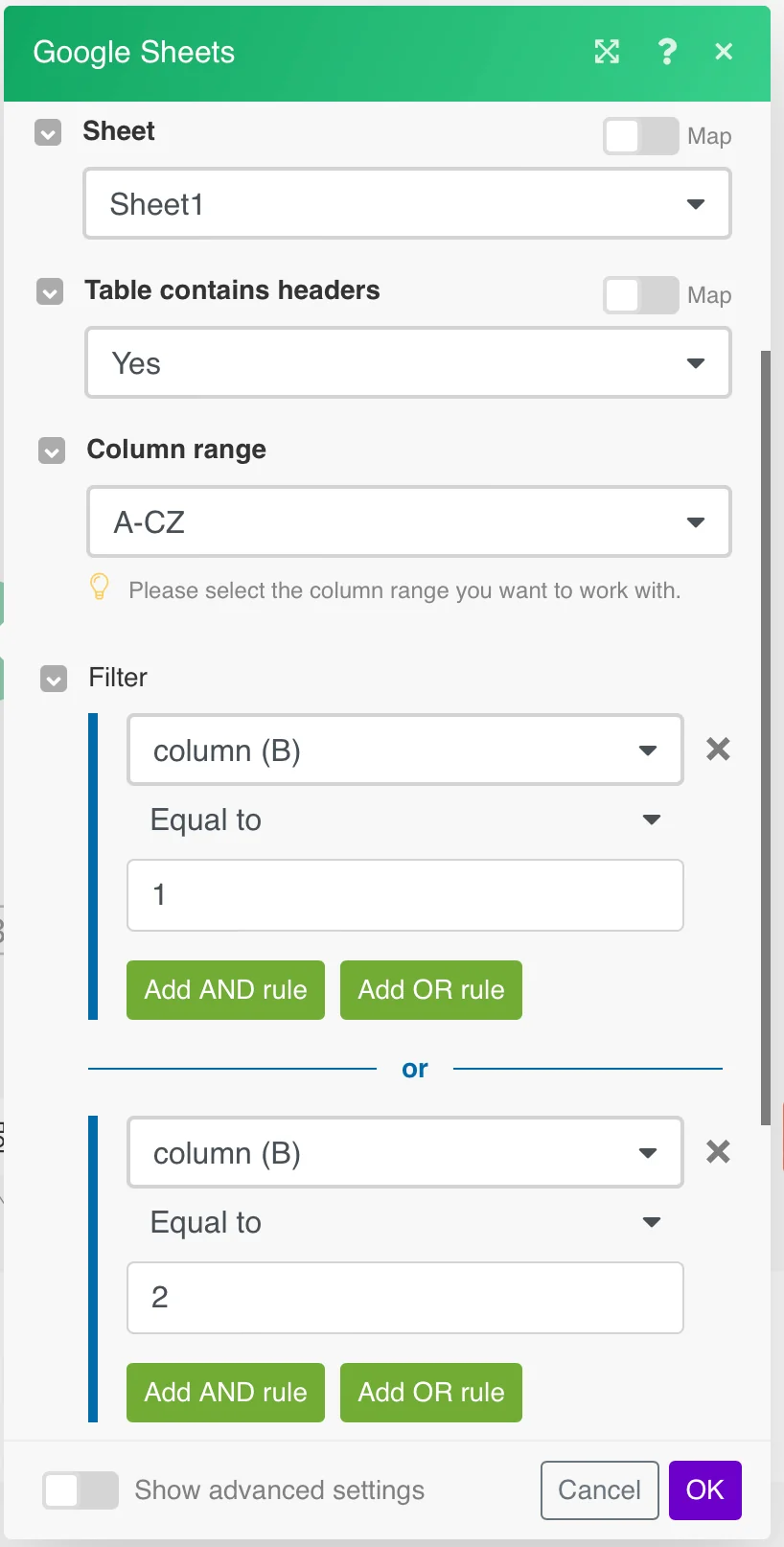
Set filter values. You can also use logical operators, AND/OR in order to specify your selection.

Example:

In the following dialog, the row which contains the number 1 or 2 in the “column2” column will be searched.

Field Type

Select or map the field type to search the rows that match the specified type:

• Date
• Number
• String

Value render option

Formatted value

The values in the reply will be calculated and formatted according to the cell’s formatting. Formatting is based on the spreadsheet’s locale, not the requesting user’s locale. For example, if A1 is 1.23 and A2 is =A1 and formatted as currency, then A2 will return "$1.23".

Unformatted value

The values will be calculated, but not formatted in the reply. For example, if A1 is 1.23 and A2 is =A1 and formatted as currency, then A2 will return the number "1.23".

Formula

The values will not be calculated. The reply will include the formulas. For example, if A1 is 1.23 and A2 is =A1 and formatted as currency, then A2 will return "=A1".

Date and time render option

Serial number

Instructs date, time, datetime, and duration fields to be output as doubles in “serial number” format, as popularized by Lotus 1-2-3. The whole number portion of the value (to the left of the decimal) counts the days since December 30th 1899. The fractional portion (to the right of the decimal) counts the time as a fraction of the day. For example, January 1st 1900 at noon would be 2.5. 2 because it’s 2 days after December 30th 1899, and .5 because noon is half a day. February 1st 1900 at 3 pm would be 33.625. This correctly treats the year 1900 as not a leap year.

Formatted string

Instructs date, time, datetime, and duration fields to be outputted as strings in their given number format (which is dependent on the spreadsheet’s locale).

Search Rows (Advanced)

Connection

Establish a connection to the spreadsheet using your Google account.

Spreadsheet

Select the Google spreadsheet.

Sheet

Select the sheet you want to search the rows in.

Query

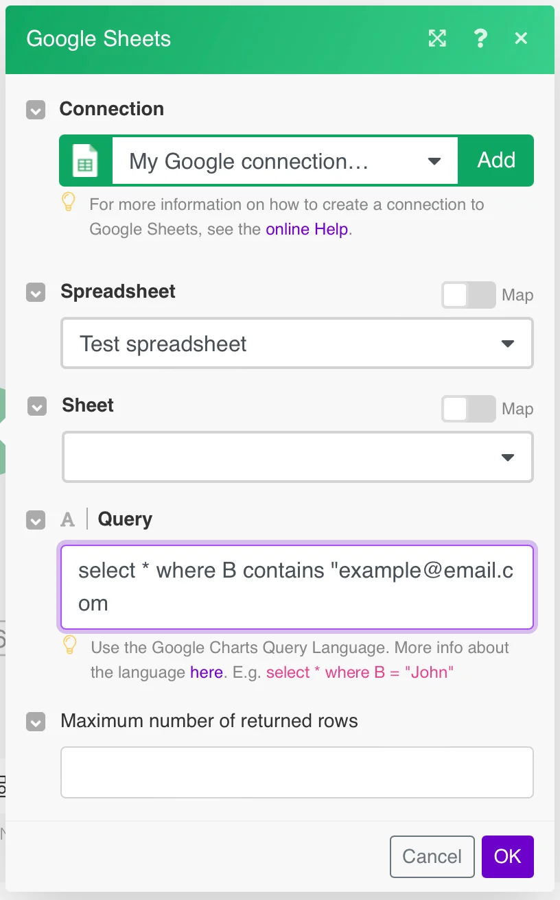
Searches rows using Google Charts Query Language. The language is similar to SQL and it is possible to make complex queries. Unfortunately, the response doesn’t contain IDs of returned rows. Due to Google Charts, the service is intended for data visualization where the row numbers aren’t needed. You can find more information about the query language in the documentation.

Get Range Values

Retrieves range content.

Connection

Establish a connection to the spreadsheet using your Google account.

Spreadsheet

Select the Google spreadsheet.

Sheet

Select the sheet you want to get the range content from.

Range

Enter the range you want to get, e.g. A1:D25.

Table contains headers

Row with headers

Enter the range of the table headers, e.g. A1:F1. If you leave the field empty, Boost.space Integrator will suppose that the header is in the first row of the specified range.

Value render option

Formatted value

The values in the reply will be calculated and formatted according to the cell’s formatting. Formatting is based on the spreadsheet’s locale, not the requesting user’s locale. For example, if A1 is 1.23 and A2 is =A1 and formatted as currency, then A2 will return "$1.23".

Unformatted value

The values will be calculated, but not formatted in the reply. For example, if A1 is 1.23 and A2 is =A1 and formatted as currency, then A2 will return the number "1.23".

Formula

The values will not be calculated. The reply will include the formulas. For example, if A1 is 1.23 and A2 is =A1 and formatted as currency, then A2 will return "=A1".

Date and render option

Serial number

Instructs date, time, datetime, and duration fields to be output as doubles in “serial number” format, as popularized by Lotus 1-2-3. The whole number portion of the value (to the left of the decimal) counts the days since December 30th 1899. The fractional portion (to the right of the decimal) counts the time as a fraction of the day. For example, January 1st 1900 at noon would be 2.5. 2 because it’s 2 days after December 30th 1899, and .5 because noon is half a day. February 1st 1900 at 3 pm would be 33.625. This correctly treats the year 1900 as not a leap year.

Formatted string

Instructs date, time, datetime, and duration fields to be outputted as strings in their given number format (which is dependent on the spreadsheet’s locale).

List Sheets

Retrieves a list of all sheets in a spreadsheet.

Connection

Establish a connection to the spreadsheet using your Google account.

Spreadsheet

Select or map the Google spreadsheet you want to retrieve sheets from.

Usage Limits

If the error 429: RESOURCE_EXHAUSTEDoccurs, you have exceeded the API rate limit.

The Google Sheets API has a limit of 500 requests per 100 seconds per project, and 100 requests per 100 seconds per user. Limits for reads and writes are tracked separately. There is no daily usage limit.

See more details at developers.google.com/sheets/api/limits.

Tips & Tricks

Deleting Multiple Rows

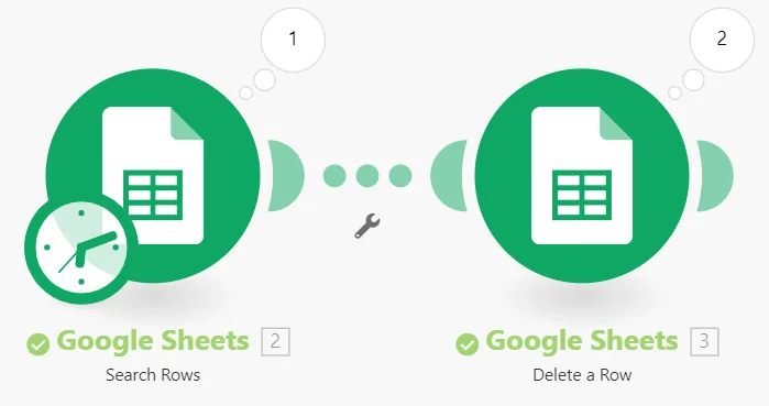
To delete multiple rows based on filter criteria use the Search Rows module linked to the Delete a Row module as on the following example:

1. 1. Add the Search Rows module and Delete a Row module to the scenario.

   

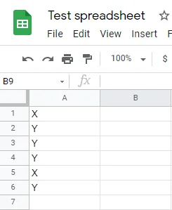
2. Let’s assume that you have a table where you need to delete all rows where column A equals to Y.

   

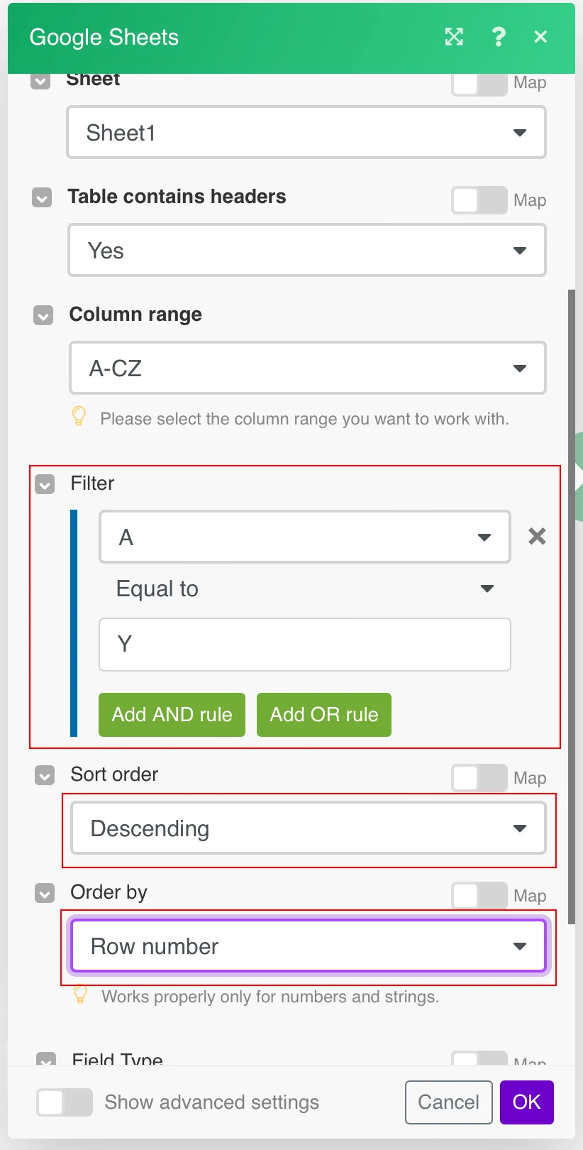
3. Open Search Rows module settings and set the fields as follows:

   Filter

   A Equal to Y

   Sort order

   Descending

   Order by

   Row number

   

Make sure that Sort order and Order by fields are set as above, otherwise, values will not be deleted correctly from the table!

4. Add the Delete a Row module to the scenario and connect it to the Search Row module.

5. Map the Row number item from the Search Rows module to the Delete a Row module’s _Row number_field.

   

6. Run the scenario to delete values that match the filter criteria from the sheet.

   

How to Get Empty Cells from a Google Sheet

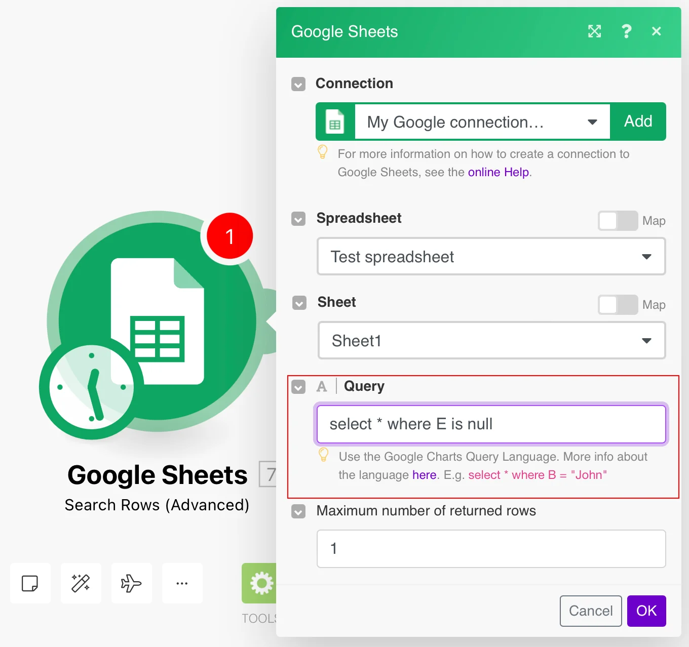
Use the Search Rows (Advanced) module & use this formula to get empty columns.

select * where E is null

Here “E” is the column & “is null” is the condition. You can create a more advanced query using Google Query Lang

Add a Custom Button in a Sheet to Trigger a Scenario

1. In Boost.space Integrator, insert the Webhook > Custom webhooks module/trigger into the scenario and configure it (see Webhooks).

2. Copy the webhook’s URL.

3. Execute the scenario.

4. In Google Sheets, choose Insert > Drawing… from the main menu bar.

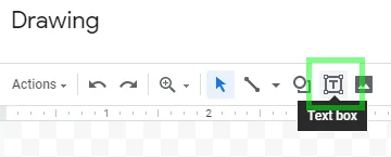
5. Click the Text box icon:

   

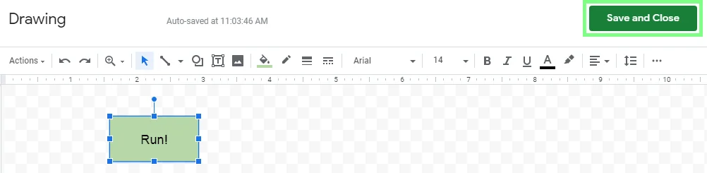
6. Design a button and click Save and Close in the top-right corner:

   

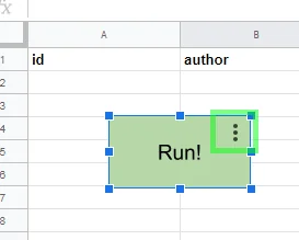
7. The button will be placed in your worksheet. Click the three vertical dots in the button’s top-right corner:

   

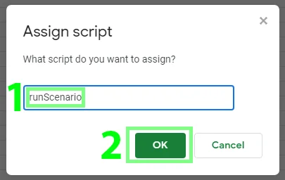
8. Choose Assign script… from the menu.

9. Enter the name of your script (function). For example, runscenarioand click OK:

   

10. Choose Tools > Script editor from the main menu bar.

11. Insert the following code:

    • The name of the function must correspond to the name you specified in step 9.

    • Replace the https://hook.make.com/xxx...xxxURL with the webhook’s URL you copied in step 2.

      function runScenario() {   UrlFetchApp.fetch("https://hook.make.com/xxx...xxx"); }
      

      plaintext

12. Press Ctrl+S to save the script file, enter a project name, and click OK.

13. Switch back to Google Sheets and click your new button.

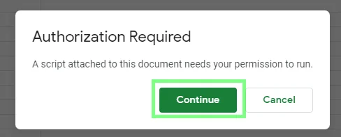
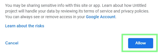
14. Grant the required authorization to the script:

    

    

15. In Boost.space Integrator, verify that the scenario has successfully executed.

Storing Dates in a Spreadsheet

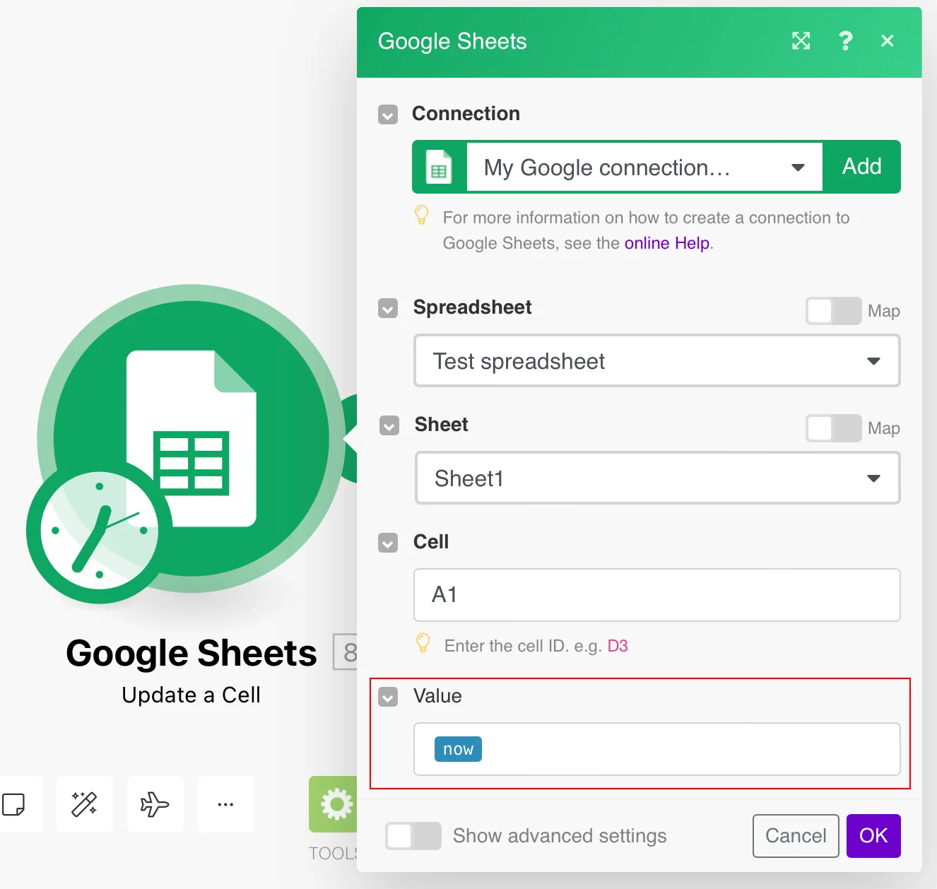
If you store a Date value in a spreadsheet without any formatting,

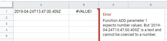
it will appear as text in ISO 8601 format in the spreadsheet. However, Google Sheets formulas or functions that work with dates do not understand this text. E.g. formula =A1+10 will display the following error:

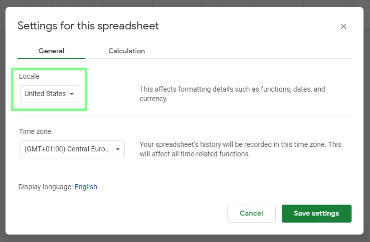
To help the GS to understand the date, format it with the formatDate(.) function. The correct format passed to the function as the second argument depends on the spreadsheet’s locale settings. Choose File ▶ Spreadsheet settings from the main menu to verify/set the locale:

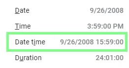
Once you have verified/set the proper locale, determine the corresponding date and time format by choosing Format ▶ Number from the main menu. The format is displayed next to the Date time menu item:

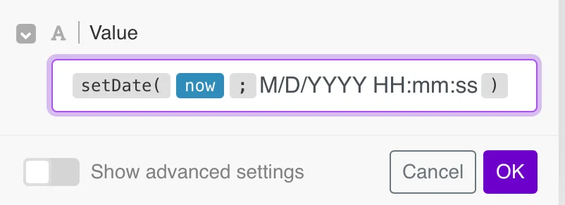
The following example shows the use of M/D/YYYY HH:mm:ss format for the United States locale:

Exploiting Google Sheets Functions

If you miss a built-in function but it is featured by Google Sheets, you may exploit it.

Posting and Getting Images from Google Sheets

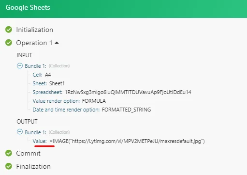
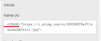
When getting an image from Google Sheets, first make sure you enter the image as a formula. For example:=IMAGE("https://i.ytimg.com/vi/MPV2METPeJU/maxresdefault.jpg") making use of the =IMAGE(…)

After you have done so, open the Google Sheets module (e.g. Watch Rows, Search Rows, Get a Cell) and select the Show advanced settings. Then select the Formula option in the Value render option_field._

The output will be as shown below:

Then you can extract the URL using the replace function.        The output will be just the URL.

To be able to post an image, make sure to enter the =IMAGE(...) formula that will be used in the cell and then enter the Image URL address.

Legacy article, imported from the original Boost.space knowledge base (/knowledge-base/applications/productivity/google-sheets/).